Guide to Using Conditional Formatting in Google Sheets

Google Sheets’ conditional formatting comes into picture when you want to highlight the data of a cell or row. It offers the opportunity to make your work easier, especially when processing large amounts of data. So whether you want to highlight a certain set of numbers or a certain type of name, you can do it right away. It also takes the hassle out of manual scanning and helps you better understand the data in front of you.

In layman’s language, conditional formatting is like a simple If-Else statement. If a criterion is met, the cell is highlighted in a certain style and ignored if not met.

In this post, we’ll show you how to use conditional formatting in Google Sheets to make your job easier. Lets start.

1. How to Use Conditional Formatting for Text

Stage 1: Select a specific column and click Format > Conditional formatting. Here, the range selected under Apply to range will be highlighted.

step 2: Next, click the drop-down list for Format rules and choose a text option. For our example data, we want to highlight all cells with items as pens.

Stage 3: Select formatting options from the menu under Formatting rules. When finished, click Done. Cells that meet the selected criteria will be highlighted in the selected color.

2. How to Use Conditional Formatting for Numbers

Stage 1: Select a data range and go to Format > Conditional formatting. You can also change the data range by clicking the table icon.

Step 2: Next, select Format rules and scroll down until you see the number options. Choose one of them and enter the value.

Next, select a formatting style and hit the Done button.

For our example sheet, we wanted to highlight cells with values ​​greater than 50. We chose the ‘greater than’ condition and added 50 to the text box. And that’s it. All cells with a value greater than 50 will be clearly highlighted.

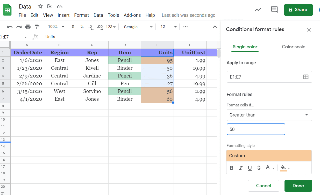
note: When it comes to numbers and numbers, defining the range is vital to get precise results. For example, if you select the entire table and then choose an ambiguous formatting rule, it will confuse the results.

Therefore, it is recommended that you choose the column (or row) wisely before continuing.

3. How to Use Conditional Formatting on Multiple Columns

Google Sheets also lets you apply the same conditional formatting to multiple columns.

Stage 1: Go to the formatting rules and click on the small table icon as shown below.

Add the first range and then click Add another range to add the second range.

For our example data, we want to highlight the contents of both columns E and F. Therefore, we chose the ranges E2 to E7 and F2 to F7.

Step 2: Once done, select a format rule along with the style from the drop-down list. You will see the data highlighted in no time.

It goes without saying that the format rule must be applied to both datasets.

4. Find All Duplicate Entries

Unfortunately, finding duplicates in a column cannot be handled by local rules. Here, you will need to add a custom rule. Fortunately, it’s not rocket science.

Stage 1: After selecting the column, scroll down in Format rules and select ‘Custom formula’.

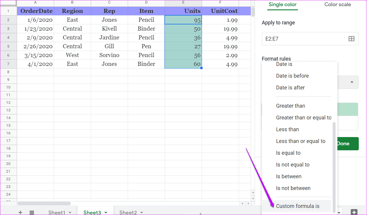
Step 2: Add the following formula to the text box.

=COUNTIF($E$2:$E$7,E2)>1 

Stage 3: Add required formatting style and have cells highlighted instantly.

If you want to highlight the whole row, adjust the formula as follows. Don’t forget to change the range to the whole table (except the header row).

=COUNTIF($E$2:$E$7,$E1)>1

Cool Tip: Simply replace ‘>’ with ‘=’ to highlight unique cells.

5. How to Highlight an Entire Row

So far, all the steps above highlight specific cells. But for a really large dataset it can be a bit overwhelming. As above, here you will have to resort to a special formula.

Stage 1: Select the table range (excluding the table header) and navigate to the Conditional formatting table. Now, under ‘Custom formula’ add the following formula,

=$E2< 30

Here we want pages to only check column E for expression. For text-based cells, the same formula works, but returns only exact matches.

=$B2 = "[text]"

Similarly, if you want to highlight the line without the word in question, replace ‘=’ with ‘<>‘.

 =$B2 <> "[text]"

6. How to Highlight a Line for Multiple Conditions

Stage 1: Select the data range. Again, make sure you don’t include the header.

Step 2: Add the following formulas under custom,

=or($B2="east", $B2="west") 

With this formula, both East and West will be searched in column B. When the expression returns a true value, the $ expression highlights the entire row.

Format Your Path

Conditional formatting in Google Sheets isn’t too hard to understand. The good news is that some formatting can be handled with local rules. While the specific rules may seem a bit overwhelming at first, it goes without saying that changing the wording makes them easier to understand.